Calibration
of an area detector in GSAS-II
In this tutorial, data collected with a Perkin-Elmer area detector at APS 11-ID-C with a wavelength 0.10798 A, where the detector was intentionally tilted at 45 degrees, are used. Note that menu entries are listed in bold face below as Help/About GSAS-II, which lists first the name of the menu (here Help) and second the name of the entry in the menu (here About GSAS-II).
If you have not done so already, start GSAS-II.
Step 1: read in the data file
Use the Import/Image/from TIF image file menu item to read the data file into the current GSAS-II project.
A file selection dialog will be shown; its appearance will depend on your OS. Change the search directory to 2DCalibration/data and then select the file
La_hex_+45deg-00015.tif
and press Open.
If the file has not been downloaded with this tutorial, it can be
found here: https://advancedphotonsource.github.io/GSAS-II-tutorials/2DCalibration/data/.

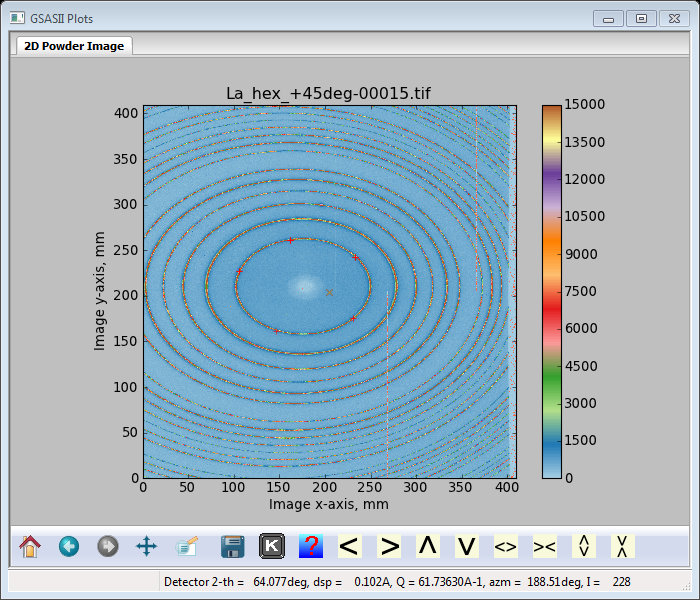
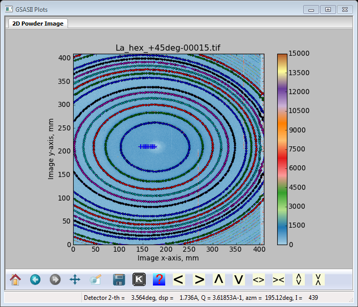
At this point the data tree window will have several entries; by default the highlighted one specifies the contents of the data window as Image Controls. I’ve expanded the window to see all the contents.
The plot window shows the image; I’ve changed the Max intensity to ~88000. Notice the elliptical shape of the powder diffraction rings due to the 45 degree detector tilt. The blue X marks the beam location (which defaults to the image center); the calibration you will perform here will find the correct placement for it. Also note that as the mouse is moved across the plot the plot window status bar (at bottom of plot window) shows the cursor position, as computed from the default (incorrect) calibration values. These constants will be correctly determined after you finish the calibration.

Step 2: Edit image parameters
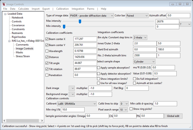
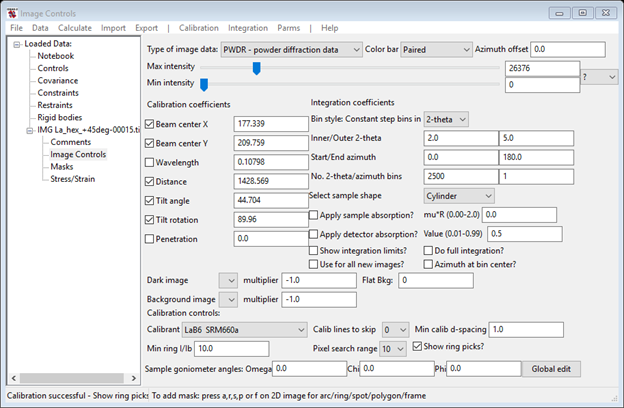
Note that, alas, very few image formats contain all of the important metadata about the image, so it needs to be added manually. In this case set the wavelength to 0.10798. We will be determining the calibration values of all the checked items. In this case wavelength is known (‘Penetration’ is a correction for x-ray penetration into the detector; it is only needed when the detector is close to the sample). Under certain circumstances it may be useful to restrict the calibration to fewer parameters (i.e. if distance is presumed to be “known”) in which case you can uncheck some of the calibration parameters and use their fixed values. It is also helpful to change the display of the image so that it is easier to see the diffraction rings. Lowering the maximum intensity to 10,000 to 20,000 counts will help (note that this can be done by moving the slider, or by typing a value in the box and then clicking on another control or pressing the Enter or Tab key). You may also wish to select another color scheme using the Color bar selector.
Step 3: Calibrate
First:
Set the material used as a sample in the box labeled Calibrant; select LaB6 SRM660a
Second:
Use the Calibration/Calibrate menu item. At this point the status line on the bottom of the Image Controls window changes with a prompt to select points for calibration.
Third:
Use the left mouse button to click on at least five locations on the innermost ring. As each point is defined, a red "+" is added to the plot. You need not hit the ring exactly as the code will search for the locally highest point in a 40x40 pixel box. (On the Mac with a two or three button mouse, also use the left mouse button, or with a standard Mac single-button mouse, use the regular mouse button.)
To remove a point added in error click on that point with the right mouse button (on the Mac, if you have a single-button mouse, hold the control key down and click). NB: it is slightly better to pick points just inside the inner ring as GSAS-II will then find the best point on that ring.
Fourth:
When done, press the right mouse button well away from any points that have been added (on the Mac, if you have a single-button mouse, hold the control key down and click).
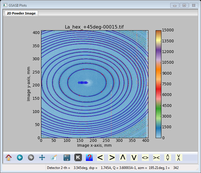
The calibration is then performed. First the rings are located and an ellipse is optimized for each ring. The indexed rings are first shown briefly in red as the calibration proceeds and center of each ellipse is noted with a blue "+"; these will track in the direction of the tilt. When all rings have been fitted, the entire ensemble of rings is refitted to the detector parameters and the rings are then shown in blue. The beam position (blue “X”) is now correctly positioned.
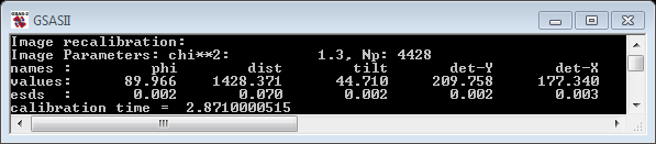
The derived calibration results are shown in the Image Controls window.
and the console window shows details of the fit.
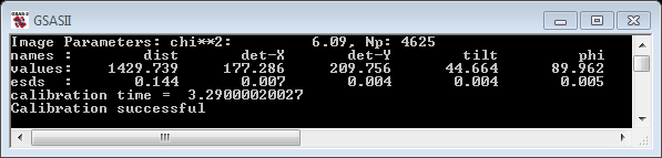
The distance is from the sample to the plane containing the detector, det-x & det-y is the incident beam location on the image, tilt is the angle of detector rotation from being normal to the incident beam and phi is the rotation of the detector tilt axis from the x-axis. To see the actual points selected by the program, click on the show ring picks? check box
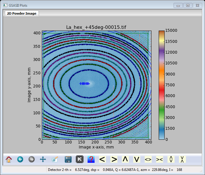
When this is done, it sometimes occurs that the points selected for the outermost rings are scattered between that and the next ring. This can be repaired by changing the pixel search range to 10 and using the Calibration/Recalibrate menu item. Also notice that the right edge of the image shows a ragged fit to the rings because of an intensity falloff. This can be removed by placing a frame mask about the “good” part of the pattern. Select the Masks GSAS-II data tree item.
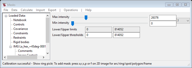
The instruction in the status bar of this frame tells you how to enter a frame: first select the plot window, then press the ’F’ key; that will “arm” the frame mask creator. Then select each corner of the good part of the image in turn (I chose points with x=400 for the right edge) with the left mouse button. After selecting the last point, close the frame with a press of the right mouse button. As each point is selected a small green ‘+’ will be drawn on the plot connected with a green line to the previous point. When you are done the image should look something like

Mask points can be moved by carefully selecting and dragging then with the left button down (you may need to zoom in to do this); the right mouse button will delete it. The Mask data window will show the new frame mask.

Now go back to the Image Controls tree item and do Calibration/Recalibrate; a better calibration will result.
Notice that the frame defined the calibration region.
And notice the better fit obtained (smaller chi**2 and smaller esds).
In cases where particular types of detectors are placed close to the sample (not the case here) and the diffraction pattern extends to near the edges of the detector, the Penetration correction may need to be refined. Just select the check box and do Calibration/Recalibrate, the result should be >0 for a reasonable correction. Close examination of the outer rings will show a small shift in the calculated rings to better match the observed ones. Assuming that these calibration results will be applied to other images to be later read into the same GSAS-II project, click on Use as default for all images. You may also save a copy of the calibration values to a file (name.imctrl) with the Parms/Save Controls menu item. To save the project, including the now-derived calibration information, use the File/Save Project menu item associated with the data tree window; as this project has not been saved before the file save dialog will need a file name. Don’t enter the extension; it will be set to “.gpx”.